  1
  2
  3
  4
  5
  6
  7
  8
  9
 10
 11
 12
 13
 14
 15
 16
 17
 18
 19
 20
 21
 22
 23
 24
 25
 26
 27
 28
 29
 30
 31
 32
 33
 34
 35
 36
 37
 38
 39
 40
 41
 42
 43
 44
 45
 46
 47
 48
 49
 50
 51
 52
 53
 54
 55
 56
 57
 58
 59
 60
 61
 62
 63
 64
 65
 66
 67
 68
 69
 70
 71
 72
 73
 74
 75
 76
 77
 78
 79
 80
 81
 82
 83
 84
 85
 86
 87
 88
 89
 90
 91
 92
 93
 94
 95
 96
 97
 98
 99
100
101
102
103
104
105
106
107
108
109
110
111
112
113
114
115
116
117
118
119
120
121
122
123
124
125
126
127
128
129
130
131
132
133
134
135
136
137
138
139
140
141
142
143
144
145
146
147
148
149
150
151
152
153
154
155
156
157
158
159
160
161
162
163
164
165
166
167
168
169
170
171
172
173
174
175
176
177
178
179
180
181
182
183
184
185
186
187
188
189
190
191
192
193
194
195
196
197
198
199
200
201
202
203
204
205
206
207
208
209
210
211
212
213
214
215
216
217
218
219
220
221
222
223
224
225
226
227
228
229
230
231
232
233
234
235
236
237
238
239
240
241
242
243
244
245
246
247
248
249
250
251
252
253
254
|
# example from https://github.com/pytorch/examples/blob/master/vae/main.py
# commented and type annotated by Charl Botha <cpbotha@vxlabs.com>
import os
import torch
import torch.utils.data
from torch import nn, optim
from torch.autograd import Variable
from torch.nn import functional as F
from torchvision import datasets, transforms
from torchvision.utils import save_image
# changed configuration to this instead of argparse for easier interaction
CUDA = True
SEED = 1
BATCH_SIZE = 128
LOG_INTERVAL = 10
EPOCHS = 10
# connections through the autoencoder bottleneck
# in the pytorch VAE example, this is 20
ZDIMS = 20
# I do this so that the MNIST dataset is downloaded where I want it
os.chdir("/home/cpbotha/Downloads/pytorch-vae")
torch.manual_seed(SEED)
if CUDA:
torch.cuda.manual_seed(SEED)
# DataLoader instances will load tensors directly into GPU memory
kwargs = {'num_workers': 1, 'pin_memory': True} if CUDA else {}
# Download or load downloaded MNIST dataset
# shuffle data at every epoch
train_loader = torch.utils.data.DataLoader(
datasets.MNIST('data', train=True, download=True,
transform=transforms.ToTensor()),
batch_size=BATCH_SIZE, shuffle=True, **kwargs)
# Same for test data
test_loader = torch.utils.data.DataLoader(
datasets.MNIST('data', train=False, transform=transforms.ToTensor()),
batch_size=BATCH_SIZE, shuffle=True, **kwargs)
class VAE(nn.Module):
def __init__(self):
super(VAE, self).__init__()
# ENCODER
# 28 x 28 pixels = 784 input pixels, 400 outputs
self.fc1 = nn.Linear(784, 400)
# rectified linear unit layer from 400 to 400
# max(0, x)
self.relu = nn.ReLU()
self.fc21 = nn.Linear(400, ZDIMS) # mu layer
self.fc22 = nn.Linear(400, ZDIMS) # logvariance layer
# this last layer bottlenecks through ZDIMS connections
# DECODER
# from bottleneck to hidden 400
self.fc3 = nn.Linear(ZDIMS, 400)
# from hidden 400 to 784 outputs
self.fc4 = nn.Linear(400, 784)
self.sigmoid = nn.Sigmoid()
def encode(self, x: Variable) -> (Variable, Variable):
"""Input vector x -> fully connected 1 -> ReLU -> (fully connected
21, fully connected 22)
Parameters
----------
x : [128, 784] matrix; 128 digits of 28x28 pixels each
Returns
-------
(mu, logvar) : ZDIMS mean units one for each latent dimension, ZDIMS
variance units one for each latent dimension
"""
# h1 is [128, 400]
h1 = self.relu(self.fc1(x)) # type: Variable
return self.fc21(h1), self.fc22(h1)
def reparameterize(self, mu: Variable, logvar: Variable) -> Variable:
"""THE REPARAMETERIZATION IDEA:
For each training sample (we get 128 batched at a time)
- take the current learned mu, stddev for each of the ZDIMS
dimensions and draw a random sample from that distribution
- the whole network is trained so that these randomly drawn
samples decode to output that looks like the input
- which will mean that the std, mu will be learned
*distributions* that correctly encode the inputs
- due to the additional KLD term (see loss_function() below)
the distribution will tend to unit Gaussians
Parameters
----------
mu : [128, ZDIMS] mean matrix
logvar : [128, ZDIMS] variance matrix
Returns
-------
During training random sample from the learned ZDIMS-dimensional
normal distribution; during inference its mean.
"""
if self.training:
# multiply log variance with 0.5, then in-place exponent
# yielding the standard deviation
std = logvar.mul(0.5).exp_() # type: Variable
# - std.data is the [128,ZDIMS] tensor that is wrapped by std
# - so eps is [128,ZDIMS] with all elements drawn from a mean 0
# and stddev 1 normal distribution that is 128 samples
# of random ZDIMS-float vectors
eps = Variable(std.data.new(std.size()).normal_())
# - sample from a normal distribution with standard
# deviation = std and mean = mu by multiplying mean 0
# stddev 1 sample with desired std and mu, see
# https://stats.stackexchange.com/a/16338
# - so we have 128 sets (the batch) of random ZDIMS-float
# vectors sampled from normal distribution with learned
# std and mu for the current input
return eps.mul(std).add_(mu)
else:
# During inference, we simply spit out the mean of the
# learned distribution for the current input. We could
# use a random sample from the distribution, but mu of
# course has the highest probability.
return mu
def decode(self, z: Variable) -> Variable:
h3 = self.relu(self.fc3(z))
return self.sigmoid(self.fc4(h3))
def forward(self, x: Variable) -> (Variable, Variable, Variable):
mu, logvar = self.encode(x.view(-1, 784))
z = self.reparameterize(mu, logvar)
return self.decode(z), mu, logvar
model = VAE()
if CUDA:
model.cuda()
def loss_function(recon_x, x, mu, logvar) -> Variable:
# how well do input x and output recon_x agree?
BCE = F.binary_cross_entropy(recon_x, x.view(-1, 784))
# KLD is Kullback–Leibler divergence -- how much does one learned
# distribution deviate from another, in this specific case the
# learned distribution from the unit Gaussian
# see Appendix B from VAE paper:
# Kingma and Welling. Auto-Encoding Variational Bayes. ICLR, 2014
# https://arxiv.org/abs/1312.6114
# - D_{KL} = 0.5 * sum(1 + log(sigma^2) - mu^2 - sigma^2)
# note the negative D_{KL} in appendix B of the paper
KLD = -0.5 * torch.sum(1 + logvar - mu.pow(2) - logvar.exp())
# Normalise by same number of elements as in reconstruction
KLD /= BATCH_SIZE * 784
# BCE tries to make our reconstruction as accurate as possible
# KLD tries to push the distributions as close as possible to unit Gaussian
return BCE + KLD
# Dr Diederik Kingma: as if VAEs weren't enough, he also gave us Adam!
optimizer = optim.Adam(model.parameters(), lr=1e-3)
def train(epoch):
# toggle model to train mode
model.train()
train_loss = 0
# in the case of MNIST, len(train_loader.dataset) is 60000
# each `data` is of BATCH_SIZE samples and has shape [128, 1, 28, 28]
for batch_idx, (data, _) in enumerate(train_loader):
data = Variable(data)
if CUDA:
data = data.cuda()
optimizer.zero_grad()
# push whole batch of data through VAE.forward() to get recon_loss
recon_batch, mu, logvar = model(data)
# calculate scalar loss
loss = loss_function(recon_batch, data, mu, logvar)
# calculate the gradient of the loss w.r.t. the graph leaves
# i.e. input variables -- by the power of pytorch!
loss.backward()
train_loss += loss.data[0]
optimizer.step()
if batch_idx % LOG_INTERVAL == 0:
print('Train Epoch: {} [{}/{} ({:.0f}%)]\tLoss: {:.6f}'.format(
epoch, batch_idx * len(data), len(train_loader.dataset),
100. * batch_idx / len(train_loader),
loss.data[0] / len(data)))
print('====> Epoch: {} Average loss: {:.4f}'.format(
epoch, train_loss / len(train_loader.dataset)))
def test(epoch):
# toggle model to test / inference mode
model.eval()
test_loss = 0
# each data is of BATCH_SIZE (default 128) samples
for i, (data, _) in enumerate(test_loader):
if CUDA:
# make sure this lives on the GPU
data = data.cuda()
# we're only going to infer, so no autograd at all required: volatile=True
data = Variable(data, volatile=True)
recon_batch, mu, logvar = model(data)
test_loss += loss_function(recon_batch, data, mu, logvar).data[0]
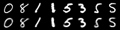
if i == 0:
n = min(data.size(0), 8)
# for the first 128 batch of the epoch, show the first 8 input digits
# with right below them the reconstructed output digits
comparison = torch.cat([data[:n],
recon_batch.view(BATCH_SIZE, 1, 28, 28)[:n]])
save_image(comparison.data.cpu(),
'results/reconstruction_' + str(epoch) + '.png', nrow=n)
test_loss /= len(test_loader.dataset)
print('====> Test set loss: {:.4f}'.format(test_loss))
for epoch in range(1, EPOCHS + 1):
train(epoch)
test(epoch)
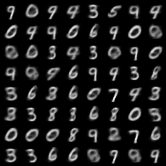
# 64 sets of random ZDIMS-float vectors, i.e. 64 locations / MNIST
# digits in latent space
sample = Variable(torch.randn(64, ZDIMS))
if CUDA:
sample = sample.cuda()
sample = model.decode(sample).cpu()
# save out as an 8x8 matrix of MNIST digits
# this will give you a visual idea of how well latent space can generate things
# that look like digits
save_image(sample.data.view(64, 1, 28, 28),
'results/sample_' + str(epoch) + '.png')
|