Post summary: The level set method is a powerful alternative way to represent N-dimensional surfaces evolving through space.

(This is a significantly extended blog-post version of three slides from my Medical Visualization lecture on image analysis.)

Imagine that you would like to represent a contour in 2D or a surface in 3D, for example to delineate objects in a 2D image or in a 3D volumetric dataset.

Now imagine that for some reason you would also like have this contour or surface move through space, for example to inflate it, or to shrink it, at the same time dynamically morphing the surface to better fit around the object of interest.

Mathematically, we would have for N dimensions the following representation:

$$ C(p,t) = \lbrace x_0(p,t), x_1(p,t), \cdots, x_{N-1}(p,t) \rbrace\tag{1} $$

Where \(C(p,t)\) is the collection of contours that you get when you morph or evolve the initial contour \(C(p,0)\) over time \(t\). At each point in time, each little bit of the contour moves orthogonally to itself (i.e. along its local normal) with a speed \(F(C(p,t))\) that is calculated based on that little bit of contour at that point in time.

This morphing of the contour can thus be described as follows:

$$ \frac{\partial C(p,t)}{\partial t} = F(C(p,t))\vec{n}(C(p,t))\tag{2} $$

In other words, the change in the contour relative to the change in time is defined by that contour- and time-dependent speed \(F\) and the normal to the contour at that point in space and time.

There are at least two ways of representing such contours, both in motion and at rest.

Contours as (moving) points in space: Explicit and Lagrangian.

Most programmers would (sooner or later) come up with the idea of using a bunch of points, and the line segments that connect them, to represent 2D contours, and, analogously, dense meshes consisting of triangles and other polygons to represent 3D surfaces, a la OpenGL.

You would be in good company if you then implemented an algorithm whereby for each iteration in time, you iterated over all points and moved each point a small distance \(F\times \Delta t\), orthogonally to the contour containing it. Such an algorithm could be called active contours, or snakes, and this way of representing a contour or surface as a collection of points moving through space is often called the Lagrangian formulation.

Now imagine that your contour or surface became quite large. You would need to add new points, or a whole bunch of new triangles. This could cause minor headaches. However, your headaches would grow in severity if your contour or surface were to shrink, and you would at some point need to remove, very carefully, extraneous points, edges or triangles. However, this headache pales in comparison to the one you would get if your surface, due to the object it was trying to delineate, would have to split into multiple surfaces, or later would have to merge back into a single surface.

Contours as (changing) measurements of the space around them: Implicit and Eulerian.

However, if you were as clever as, say James Sethian and Stanley Osher, you would decide to sidestep all of that headache and represent your contour implicitly. This can be done by creating a higher-dimensional embedding function or level set function of which the zero level set, or the zero-valued isocontour, is the contour that you’re trying to represent. This is often called the Eulerian formulation, because we’re focusing on specific locations in space as the contour moves through them.

Huh?

(that was what I said when I first read this.)

What’s an isocontour? That’s a line, or a surface (or a hyper-surface in more than 3D) that passes through all locations containing the isovalue. For example, on a contour map you have contour lines going through all positions with the same altitude.

If I were to create a 2D grid, with at each each grid position the floating point closest distance to a 2D contour (by convention, the distance inside the contour is negative and outside positive), then the contour line at value zero (or the zero level set) of that 2D grid would be exactly the 2D contour!

The 2D grid I’ve described above is known as an embedding function \( \phi(x,t)\) of the 2D contour. There are more ways to derive such embedding functions, but the signed distance field (SDF) is a common and practical method.

Let’s summarise what we have up to now: Instead of representing a contour as points, or a surface as triangles, we can represent them as respectively a 2D or 3D grid of signed distance values

For the general case up above, the contour at fixed time \(t_i\) would be:

$$ C(t_i) = \lbrace x \vert \phi(x,t_i) = 0 \rbrace $$

Moving contours are simply point-wise changes in their embedding functions

Instead of directly evolving the contour, it can be implicitly evolved by incrementally modifying its embedding function. Given the initial embedding function \(\phi(x,t=0)\), the contour can be implicitly evolved as follows:

$$ \frac{\partial \phi(x,t)}{\partial t} = – F(x,t) \lvert \nabla \phi(x,t) \rvert $$

where \(F(x,t)\) is a scalar speed function, \(\nabla\) is the gradient operator and \(\lvert \nabla \phi(x,t) \rvert\) is the magnitude of the gradient of the level set function. Note the similarity with the general contour evolution equation 2 above.

In practice, this means that for each iteration, you simply raster scan through the embedding function (2D, 3D or ND grid), and for each grid position you calculate speed \(F(x,y)\), multiply with the negative gradient magnitude of the embedding function, and then add the result to whatever value you found there.

If you were to extract the zero level set at each iteration, you would see the resultant contour (or surface) deform over time according to the speed function \(F\) that you defined.

MAGIC!

A visual confirmation

The figure below is a signed distance field representing two concentric circles in 2D, or a 2D donut. Note that the values are negative inside the donut, and positive elsewhere (in the center of the image, and towards the limits of the grid).

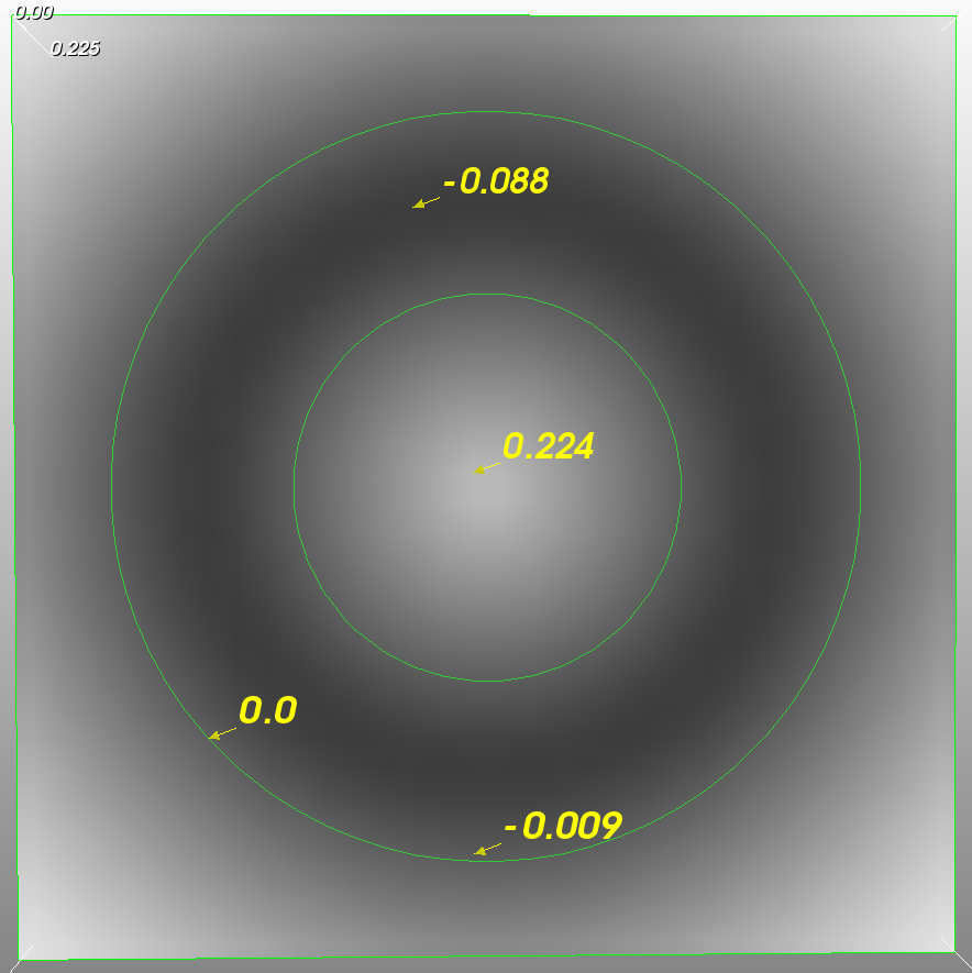
For the sake of this exposition, let’s define \(F(x,t)=1\), i.e. the donut should get fatter over time. Eventually it will get so fat that the hole in the middle will be closed up.

You can now check by inspection that at each point in the embedding function, or the image, you would have to add a small negative number (\(-1\) multiplied by the gradient magnitude). First positive regions close to the contour will become negative, increasing its size, and regions further away will approach zero from above, and eventually also become negative, making the donut even fatter. Eventually the region in the middle will become all negative, in other words, close up.

Conclusion

Representing surfaces implicitly, and specifically as signed distance fields, has numerous advantages.

• Contours always have sub-grid-point resolution.
• Topological changes, such as splitting and merging of N-dimensional objects, is automatically handled.
• Implementation of N-dimensional contour propagation becomes relatively straight-forward.
• With this implicit representation, morphing between two N-dimensional contours is a simple point-wise weighted interpolation!

Although iterating through the embedding function is much simpler than managing a whole bunch of triangles and points moving through space, it can be computationally quite demanding. A number of optimization techniques exist, mostly making use of the fact that one only has to maintain the distance field in a narrow region around the evolving contour. These are called narrow-band techniques.

The Insight Segmentation and Registration ToolKit, or ITK, has a very good implementation of a number of different level set method variations. You can also use the open source DeVIDE system to experiment with level set segmentation and 3D volumetric datasets (it makes use of ITK for this).

(I’m planning to make available my MedVis post-graduate lecture exercises. Let me know in the comments how much I should hurry up.)